Predicting the interest rate

Our goal in this assignment is to predict the interest rate of government debt as accurately as possible.

Outcomes

Fit statistical learning models to multivariate data
Create numeric variables from character vectors
Compare test set performance of different models

Instructions

Answer the following questions, and show all your R code.
Upload your submission to Canvas in nicely formatted HTML generated from Rstudio.

Data

The California DebtWatch contains the following information:

The principal amounts, sale dates, interest rates, terms, purposes, ratings, costs of issuance, financing team participants, issuance documents, and annual reporting (if applicable), among 67 other data points required under California Government Code section 8855, of the various types of debt issued by all state and local government agencies in California.

Download the data in CSV format and load it into R. Randomly select 20% of the rows and save them into a test set to use later to evaluate the performance of your model. Which column(s) represent interest rate?

set.seed(280)
debt = read.csv("C:/Users/kanni/Downloads/CDA_ALL_Raw.csv")
dim(debt)

## [1] 67043    68

debt20 = debt[sample(nrow(debt), round(0.2*67043)), ]
dim(debt20)

## [1] 13409    68

debt80 = debt[sample(nrow(debt), round(0.8*67043)), ]
dim(debt80)

## [1] 53634    68

grep("interest.rate", colnames(debt80), ignore.case = TRUE, value = TRUE)

## [1] "TIC.Interest.Rate" "NIC.Interest.Rate"

Calculated Columns

Define one or more new columns from existing text columns in the data set. For example, you could add a logical column indicating whether the term “lease” appears in some column. Why do you think this new column will help you improve the accuracy of your model?

rate = rep(0, times = nrow(debt80))
rate[!is.na(debt80$TIC.Interest.Rate) & is.na(debt80$NIC.Interest.Rate)] = debt80$TIC.Interest.Rate

## Warning in rate[!is.na(debt80$TIC.Interest.Rate) &
## is.na(debt80$NIC.Interest.Rate)] = debt80$TIC.Interest.Rate: number of items to
## replace is not a multiple of replacement length

rate[is.na(debt80$TIC.Interest.Rate) & !is.na(debt80$NIC.Interest.Rate)] = debt80$NIC.Interest.Rate

## Warning in rate[is.na(debt80$TIC.Interest.Rate) & !
## is.na(debt80$NIC.Interest.Rate)] = debt80$NIC.Interest.Rate: number of items to
## replace is not a multiple of replacement length

rate[is.na(debt80$TIC.Interest.Rate) & is.na(debt80$NIC.Interest.Rate)] = NA
debt80$rate = rate

summary(debt80$TIC.Interest.Rate)

##    Min. 1st Qu.  Median    Mean 3rd Qu.    Max.    NA's 
##   0.000   2.656   4.022   4.192   5.950  71.468   26409

summary(debt80$NIC.Interest.Rate)

##    Min. 1st Qu.  Median    Mean 3rd Qu.    Max.    NA's 
##   0.000   2.868   4.271   4.393   6.200  63.037   16837

summary(debt80$rate)

##    Min. 1st Qu.  Median    Mean 3rd Qu.    Max.    NA's 
##   0.000   0.000   0.000   2.384   4.486  63.037   17763

Models

Use the remaining 80% of the data (the training set) to come up with two different models to predict interest rate. You’re welcome to use any external machine learning libraries you like, or you can stick with the lm and rpart from class. Note that you can come up with different models by using different subsets of columns. For example, a model with 3 input columns differs from a model with 60 input columns. Briefly describe the two models you ended up with.

library(rpart)
debt80$by.Year = as.POSIXct(debt80$Sale.Date, format = "%m/%d/%Y %H:%M:%OS %p")
fit1 = rpart(rate ~ Principal.Amount, data = debt80)
fit2 = lm(rate ~ by.Year, data = debt80)

length(debt80$Principal.Amount)

## [1] 53634

length(debt80$rate)

## [1] 53634

length(debt80$by.Year)

## [1] 53634

plot(debt80$Principal.Amount, debt80$rate)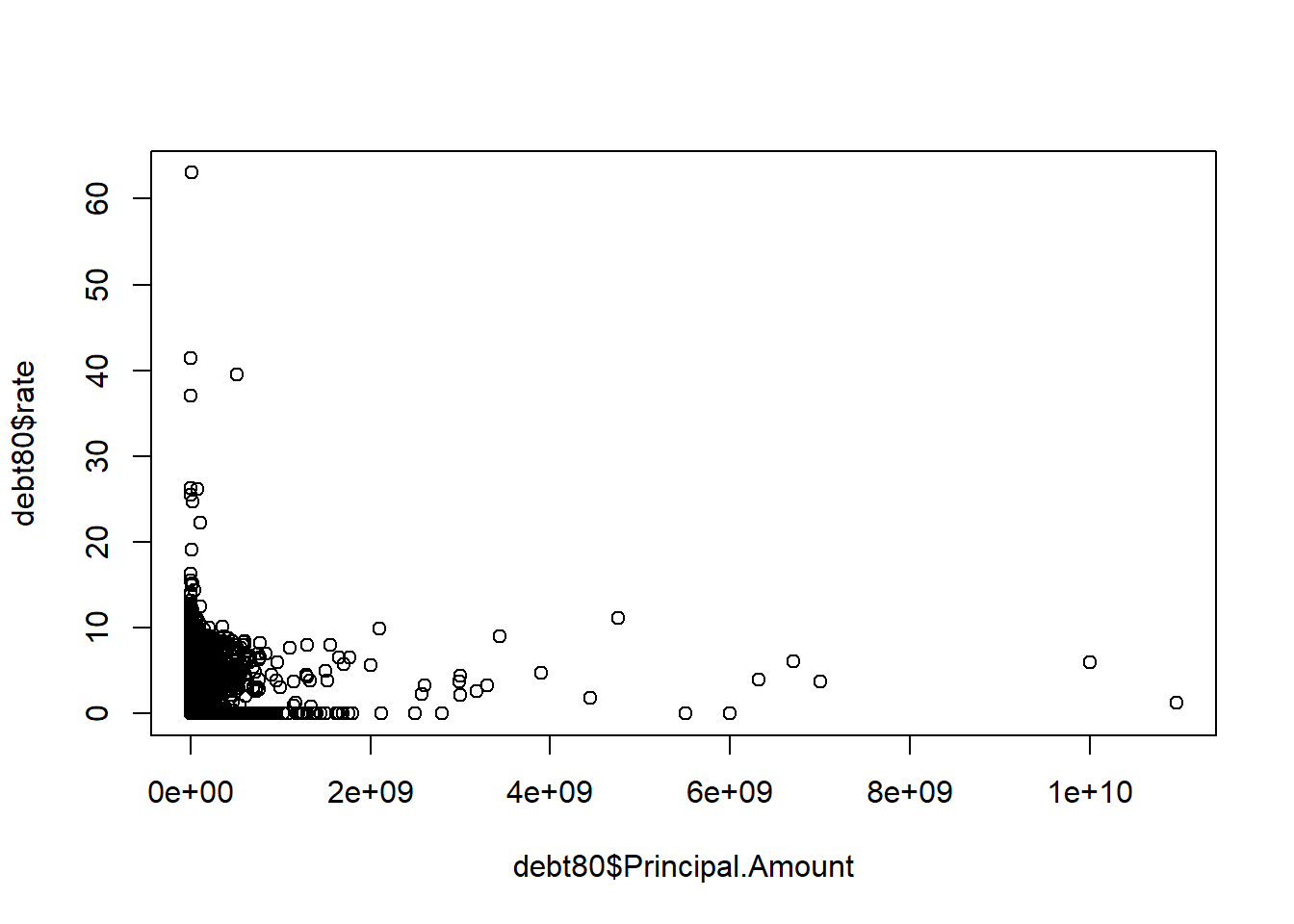

#lines(debt80$Principal.Amount,predict(fit1), col = "blue",lwd = 2)

plot(debt80$by.Year, debt80$rate)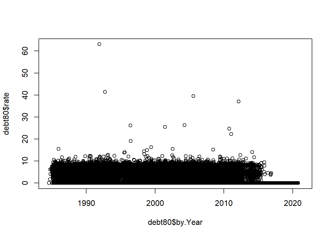

#lines(debt80$by.Year,predict(fit2), col = "green",lwd = 2)

Evaluating Performance

Evaluate both of your models on the 20% of the data you reserved for the test set by looking at the average absolute difference between the interest rate predicted by the model and the actual interest rate. Do the models do a reasonable job of predicting interest rate? Find the rows where the predicted interest rate is farthest from the true interest rate. Why might the model have done a poor job on these rows?